
The word2vec model, introduced by Google researchers in 2013, revolutionized how we represent language using dense vector embeddings. This post revisits the Continuous Bag of Words (CBOW) architecture of word2vec, implementing it in JAX and comparing it to the original C version.
Understanding Embeddings
In NLP, word embeddings are dense vectors that encode the semantic meaning of words such that similar words are close in vector space. Unlike sparse one-hot vectors, embeddings are compact and meaningful, enabling downstream tasks like classification, clustering, or analogy solving.
The CBOW Architecture
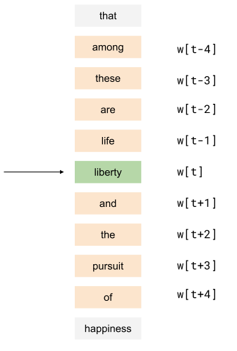
CBOW learns to predict a word from its surrounding context. For example, given the context ["the", "statue", "of", "liberty", "is", "in", "new", "york"], the model should predict the center word (e.g. "liberty").
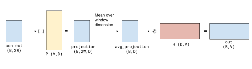
Architecture summary:
- Input: Batch of context word indices → shape
(B, 2W) - Projection matrix: Embedding lookup from shape
(V, D)→ result(B, 2W, D) - Averaging: Compute mean over context →
(B, D) - Output: Dense vector passed through hidden weights
(D, V)→ logits(B, V) - Loss: Softmax cross-entropy against the one-hot target
JAX Implementation
Forward Pass
python @jax.jit
def word2vec_forward(params, context):
    projection = params["projection"][context]  # (B, 2W, D)
    avg_projection = jnp.mean(projection, axis=1)  # (B, D)
    return jnp.dot(avg_projection, params["hidden"])  # (B, V)
Loss Function
python @jax.jit
def word2vec_loss(params, target, context):
    logits = word2vec_forward(params, context)
    target_onehot = jax.nn.one_hot(target, logits.shape[1])
    return optax.softmax_cross_entropy(logits, target_onehot).mean()
Data Preprocessing
Using the classic text8 dataset, preprocessing includes:
Subsampling Frequent Words
python def subsample(words, threshold=1e-4):
    freqs = Counter(words)
    total = len(words)
    keep_prob = {
        w: math.sqrt(threshold / (c / total)) if c / total > threshold else 1.0
        for w, c in freqs.items()
    }
    return [w for w in words if random.random() < keep_prob[w]]
Building the Vocabulary
python def make_vocabulary(words, top_k=20000):
    vocab = {"<unk>": 0}
    for word, _ in Counter(words).most_common(top_k - 1):
        vocab[word] = len(vocab)
    return vocab
Training Loop
Training closely mirrors the original hyperparameters:
python def train(train_data, vocab):
    V, D, W, BATCH, EPOCHS = len(vocab), 200, 8, 1024, 25
    params = {
        "projection": initializer(jax.random.PRNGKey(0), (V, D)),
        "hidden": initializer(jax.random.PRNGKey(0), (D, V)),
    }
    opt = optax.adam(1e-3)
    opt_state = opt.init(params)

    for epoch in range(EPOCHS):
        for target_batch, context_batch in generate_train_vectors(train_data, vocab, W, BATCH):
            loss, grads = jax.value_and_grad(word2vec_loss)(params, target_batch, context_batch)
            updates, opt_state = opt.update(grads, opt_state)
            params = optax.apply_updates(params, updates)
Embedding Usage & Word Similarities
After training, the learned projection matrix P contains the final word embeddings. Use cosine similarity to find nearest neighbors or solve analogies:
bash $ python similar-words.py -word paris -checkpoint checkpoint.pickle
Words similar to 'paris':
paris     1.00
france    0.50
french    0.49
toulouse  0.38
Word Analogy Example:
bashКопіюватиРедагувати$ python similar-words.py -analogy berlin,germany,tokyo
Analogies:
tokyo     0.70
japan     0.45
osaka     0.40
Original C Code
The original word2vec C implementation is available via GitHub mirror. Despite being over a decade old, it compiles and runs easily with make, enabling quick comparisons to the JAX version.
Modern Embeddings in LLMs
While word2vec was foundational, modern LLMs like GPT train embeddings jointly with their tasks (e.g. token prediction). Differences include:
- Embedding tokens, not words
- Much deeper embeddings (e.g. GPT-3 uses D = 12288)
- Trained end-to-end rather than standalone
Final Thoughts
Reproducing word2vec in JAX is a great exercise in understanding early NLP embeddings. While mostly of historical interest today, it still serves as a useful tool for learning about vector semantics and efficient model training.


